Time courses
Grid of 1000-sample bins (10.0 s). Column k holds the events up to and including sample k × 1000 (MATLAB cumsum(...)(1:SFactor:end)). Curves = mean ± SEM over flies (SEM = sample SD / sqrt(n)).
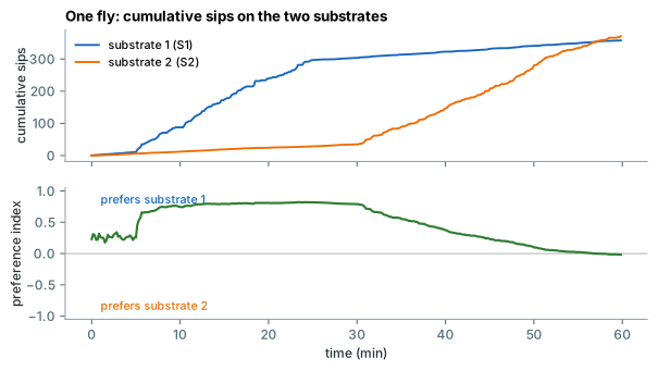
Cumulative sips / feeding bursts
Number of sip (burst) onsets up to the end of the bin. For a recording shorter than the analysis duration the bins after its end are empty (no data), not 0, and are left out of the group mean/median.
InterpretationTime course of intake; the slope is the feeding rate.
Where: Cumulative plots, Cumulative*InExcelFormat.xlsx
Code:
analysis/cumulative.py::compute_cumulative_events · fingerprint 69903d3cb515Cumulative activity
Active samples up to the end of the bin / 100. Bins after the end of a shorter recording are empty (no data), as for cumulative sips.
InterpretationTime course of engagement with the food.
Code:
analysis/cumulative.py::compute_cumulative_events · fingerprint 69903d3cb515Non-cumulative (per bin)
Difference of consecutive cumulative values (first bin = its own value).
InterpretationInstantaneous rate; shows satiation (decline) or late feeding.
Code:
analysis/cumulative.py::compute_non_cumulative_rates · fingerprint cc8e1b6009ebPreference index (sips, activity)
(S1 – S2) / (S1 + S2 + 2) with S = cumulative (or per-bin) value of substrate 1 / 2 of the same fly (MATLAB adds 1 to each count). Flies are paired explicitly; a fly missing one substrate is left out. Bins without data (after a shorter recording's end) are left out of the mean/median. When conditions have their own food pairs, each condition's PI compares its own two foods (legend: C01 (1 mM vs 2 mM)).
Interpretation+1 = only substrate 1, -1 = only substrate 2, 0 = no preference or no feeding. The +2 pulls values of flies with few events towards 0.
Where: Preference index plots, *PIInExcelFormat.xlsx
Code:
analysis/preference_index.py::compute_preference_index, analysis/cumulative.py::_summarise · fingerprint 752f4ca823bdTime-resolved per-fly parameters
Number of transitions, median transition IBI, median activity bout duration and median bout IBI per bin (events assigned to the bin of their time sample), cumulative and per bin. One row per fly, one column per 10-s bin; recordings longer than 45.5 h (more bins than Excel's 16,384 columns) get the same grids as CSV files in TimeResolvedCSV/, one per sheet.
InterpretationChanges of visit and switching behaviour over the recording.
Where: Cumulative/NONCumulative*InExcelFormat.xlsx, FlyIndexInExcelFormat.xlsx
Code:
export/extra_outputs.py::export_extra_time_resolved, export/extra_outputs.py::bin_events_to_grid · fingerprint e2a600eeb198Substrate transitions (two substrates)
Only for configurations with two substrates per fly.
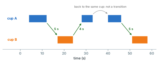
Transition IBI
For each activity bout offset on one substrate: the time to the next bout onset on the other substrate, counted only if the fly reaches the other substrate before its own next bout on the same substrate.
InterpretationTravel time between the two foods when switching; the number of transitions measures switching between foods (exploration / choice).
Code:
analysis/statistics.py::compute_transition_metrics, export/extra_outputs.py::transitions · fingerprint dd519f804342Number of transitions / median transition IBI
Per fly: number of transition IBIs (0 if none) and their median (left out if none), for substrate 1 → 2 and 2 → 1.
InterpretationFrequency and speed of switching.
Where: Transition IBIs plot
Code:
analysis/statistics.py::compute_transition_metrics · fingerprint 4fe961c25f12Visit sequence / transition matrix
Activity bouts of both cups in time order as visits A/B; counts and probabilities of A→A, A→B, B→A, B→B. With per-condition food pairs, the food names in the tables are those of the fly's condition.
InterpretationStructure of food choice over time (staying vs switching).
Where: TransitionSequence*.xlsx/csv, TransitionMatrixInExcelFormat.xlsx
Code:
export/extra_outputs.py::export_transition_sequences · fingerprint be4c0fb2bf42Distributions
Sip duration / inter-sip interval histograms
Per fly: MATLAB hist(x, 1:50) – bin centres 1..50 samples (10-500 ms), values outside counted in the end bins (the last bin therefore also holds everything > 0.5 s). Curves = mean ± SEM over all flies (flies without sips count as zeros).
InterpretationShape of the sip and rhythm distributions (e.g. a peak shift = slower rhythm). The last bin is inflated by long values by design.
Where: Histogram plots, Sip*HistogramsInExcelFormat.xlsx
Code:
analysis/distributions.py::matlab_hist, analysis/distributions.py::compute_grouped_histograms, analysis/distributions.py::collect_per_fly_histograms · fingerprint 0245fcda189cCCDF
1 – empirical CDF of all values of a condition (plot currently disabled).
InterpretationTail of distributions on log scales.
analysis/distributions.py::compute_ccdf · fingerprint ccdca7dfcfa5